推荐系统:基本件

分布变换

q_adjuster

xx变换

有时模型预估值分布得较为密集，为了让不同的item更有区分性，方便下游使用，经常用一些函数变换来分布。这里列一些常用的。

一种是拉伸q值较小部分的： \[ q_{adjust} = \frac{q * (1+\text{factor})}{1+\text{factor} * q} \] 其中factor越接近于0，变换后的分布越等价于不变，越大越拉伸q值较小的部分，一般用1.5就差不多了。

指数变换

控制该q值在所有因子中的作用力度，alpha越大，力度越大： \[ q_{adjust} = e^{\alpha * \text{Norm}(q)} \]

norm

类别

除以q的均值

• TODO：尝试从data_norm（Instance Normalization）的角度去理解一下

batch norm

参考：https://kexue.fm/archives/6992

RMS Norm

layer norm

group layer norm

norm位置

Post-Norm

残差设计作为深度网络的标配，设x的方差是\(\sigma_1^2\)，设F(x)的方差是\(\sigma_2^2\)，并且假设两者互相独立，那么x+F(x)的方差为\(\sigma_1^2 + \sigma_2^2\)，随着层数加深，输出层的方差将呈指数级增长，即残差结构会放大方差。考虑到『当输出数值方差过大时，容易导致在模型中的某一层变成接近onehot而梯度消失』，需要缩小其方差。

最直接的方案是在残差后加Norm，保证每次残差操作后输出层的方差都重新标准化到1上： \[ \begin{align} x_{t+1} &= \text{Norm}(x_t + F_t(x_t)) \\ &= \text{Norm}(\text{Norm}(x_{t-1} + F_{t-1}(x_{t-1})) + F_t(x_t)) \\ &= \text{Norm}(\text{Norm}\textcolor{blue}(\text{Norm}^{...}\textcolor{red}(x_{0} + F_{0}(x_{0})\textcolor{red}) + ... + F_{t-1}(x_{t-1})\textcolor{blue}) + F_t(x_t)) \end{align} \] 但从上式能很明显地看出，恒等分支传到t+1层时，其量级已被指数级缩小（设每一层的标准差都为2，那么传到t+1层时，\(x_0\)已被缩小\(2^{t+1}\)倍），相当于削弱了恒等分支，每Norm一次就削弱一次恒等分支的权重。即Post-Norm的梯度流会更侧重于残差分支。故在较深的网络中，Post-Norm容易导致梯度消失（gradient vanishing），模型难以训好。

当然这是模型参数初始化问题，是一个收敛难易的问题，而非模型拟合能力的问题。若训练后x+F的标准差是小于1的数，那么Norm的操作便会放大恒等分支的权重，所以如果模型能较好地收敛，那也没啥问题。

参考：https://kexue.fm/archives/8620#%E6%AE%8B%E5%B7%AE%E8%BF%9E%E6%8E%A5

Pre-Norm

为保证残差的恒等映射，Pre-Norm采用什么时候用什么时候做Norm的方案，即保证了恒等映射，又避免了方差呈指数级增长（Pre-Norm的方差随模型深度线性增长）： \[ \begin{align} x_{t+1} &= x_t + F_t(\text{Norm}(x_t)) \\ &= x_{t-1} + F_{t-1}(\text{Norm}(x_{t-1})) + F_{t}(\text{Norm}(x_{t})) \\ &= x_{0} + F_{0}(\text{Norm}(x_{0})) + ... + F_{t-1}(\text{Norm}(x_{t-1})) + F_{t}(\text{Norm}(x_{t})) \end{align} \] 但依然会存在问题。因为Norm的存在，后面的各项应该量级相同（若为一个合理的模型， \(F_0、...、F_t\) 这些函数变换应该在相同的量级上），故当 t 较大时，便有（类似于100+1≈100）： \[ \begin{align} x_{t} &= x_{0} + F_{0}(\text{Norm}(x_{0})) + ... + F_{t-2}(\text{Norm}(x_{t-2})) + F_{t-1}(\text{Norm}(x_{t-1})) \\ &\approx x_{0} + F_{0}(\text{Norm}(x_{0})) + ... + F_{t-2}(\text{Norm}(x_{t-2})) \\ &= x_{t-1} \end{align} \] 故： \[ \begin{align} x_{t+1} &= x_{t-1} + F_{t-1}(\text{Norm}(x_{t-1})) + F_{t}(\text{Norm}(x_{t})) \\ &\approx x_{t-1} + F_{t-1}(\text{Norm}(x_{t-1})) + F_{t}(\text{Norm}(x_{t-1})) \end{align} \] 即，当层数较深时，Pre-Norm相当于把模型变宽了，模型的深度没怎么增加。即Pre-Norm的梯度流会更侧重于恒等分支。故在较深的网络中，Pre-Norm容易导致表征坍缩（representation collapse），即深层表示过于相似，额外层的贡献逐渐减弱，从而削弱了模型学习能力。

与Post-Norm不同，Pre-Norm的设置便是模型拟合能力的问题了。

参考：https://kexue.fm/archives/9009

HC

Post-Norm与Pre-Norm两者取其中，几个Pre-Norm后加一个Post-Norm，以此权衡梯度消失与表征坍缩的问题，算是最直接的方案。

这个权衡问题，本质上权衡的是什么呢？Post-Norm与Pre-Norm预设了残差层的输出与输入的连接强度，本质上权衡的就是这个连接强度。

mHC

门控机制

element-wise multi

做gate时，用于计算gate的特征一般要先freeze掉：避免互相影响。

gate输出的值，一般都用[-15, 15]截断后过sigmoid再乘个2：正则化&保持输出的期望为1。

feild gate

poso

senet

ppnet、epnet都属于这种。

cgc

attention（transformer）

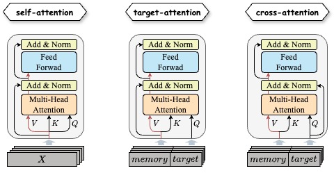
MHA的计算逻辑为： \(\text{softmax}(Q \times K^T + mask) \times V\) ，实现示例如下：

class MultiHeadAttention(paddle.nn.Layer):
    def __init__(self, d_model, num_heads, dropout=0.1, need_weights=False, name_scope='MHA01'):
        super(MultiHeadAttention, self).__init__()
        assert d_model % num_heads == 0, "d_model must be divisible by num_heads"
        
        self.d_model = d_model
        self.num_heads = num_heads
        self.head_dim = d_model // num_heads
        self.dropout = dropout
        self.need_weights = need_weights

        self.W_q = paddle.nn.Linear(d_model, d_model,
                                    weight_attr=paddle.ParamAttr(name=f'{name_scope}_Q.w_0', initializer=paddle.nn.initializer.Normal(mean=0.0, std=0.02)),
                                    bias_attr=paddle.ParamAttr(name=f'{name_scope}_Q.b_0'))
        self.W_k = paddle.nn.Linear(d_model, d_model,
                                    weight_attr=paddle.ParamAttr(name=f'{name_scope}_K.w_0', initializer=paddle.nn.initializer.Normal(mean=0.0, std=0.02)),
                                    bias_attr=paddle.ParamAttr(name=f'{name_scope}_K.b_0'))
        self.W_v = paddle.nn.Linear(d_model, d_model,
                                    weight_attr=paddle.ParamAttr(name=f'{name_scope}_V.w_0', initializer=paddle.nn.initializer.Normal(mean=0.0, std=0.02)),
                                    bias_attr=paddle.ParamAttr(name=f'{name_scope}_V.b_0'))
        self.W_o = paddle.nn.Linear(d_model, d_model,
                                    weight_attr=paddle.ParamAttr(name=f'{name_scope}_O.w_0', initializer=paddle.nn.initializer.Normal(mean=0.0, std=0.02)),
                                    bias_attr=paddle.ParamAttr(name=f'{name_scope}_O.b_0'))

    def split_heads(self, x):
        """ split_heads """
        x = paddle.reshape(x=x, shape=[0, 0, self.num_heads, self.head_dim])
        x = paddle.transpose(x=x, perm=[0, 2, 1, 3])
        return x

    def scaled_dot_product_attention(self, Q, K, V, mask=None):
        """
        通过对Q、K选择不同的src, 实现不同效果的注意力机制, 即attention_weights.
        所谓注意力, 其实就是对V的线性组合系数(V中的行向量是各位置的原始向量).
        attention_weights作用的实现方式(矩阵乘积):
          - 从『对两个矩阵各列向量的inner product的陈列』的视角去看.
                           $ w_i^T V $
            即, attention_weights的第i行代表的是, 计算第i个位置的
            表征时, 对V中各位置原始向量的线性组合系数.
          - mask是通过attention_weights作用的, 在线性组合各位置向
            量时, 将某些位置的系数置零, 从而实现输出的第i个位置的表征
            不依赖某些位置, 即所谓的看不见.
        """
        scores = paddle.matmul(x=Q * (self.head_dim**-0.5), y=K, transpose_y=True)
        if mask is not None:
            mask = _convert_attention_mask(mask, scores.dtype)
            scores = scores + mask
        # 序列维度聚合权重的约束: \sum{scores} = 1
        # attention_weights = F.softmax(scores)
        attention_weights = F.sigmoid(scores)
        if self.dropout:
            attention_weights = F.dropout(attention_weights,
                                self.dropout,
                                mode="upscale_in_train")
        output = paddle.matmul(attention_weights, V)
        return output, attention_weights

    def forward(self, query, key, value, mask=None, cache=None):
        """
        Applies multi-head attention to map queries and a set of key-value pairs to outputs.
        """
        Q = self.W_q(query)  # (batch_size, seq_len, d_model)
        K = self.W_k(key)
        V = self.W_v(value)
        
        Q = self.split_heads(Q)  # (batch_size, num_heads, seq_len, head_dim)
        K = self.split_heads(K)
        V = self.split_heads(V)
        
        attention_output, attention_weights = self.scaled_dot_product_attention(Q, K, V, mask)

        attention_output = paddle.transpose(attention_output, perm=[0, 2, 1, 3])
        concat_output = paddle.reshape(x=attention_output, shape=[0, 0, attention_output.shape[2] * attention_output.shape[3]])
        
        output = self.W_o(concat_output)  # (batch_size, seq_len, d_model)

        outs = [output]
        if self.need_weights:
            outs.append(attention_weights)
        return output if len(outs) == 1 else tuple(outs)

• Q、K、V的形状均为 [batch_size, num_heads, seq_len, head_dim]
• 简略为 \((QK^T)V\) 以便说明：
  • 括弧外为第一部分，即attention的操作，其实就是对V中的向量做各种不同权重的线性组合（V中的行向量为各位置的”原始向量”）；attention_weights的第i行代表的是，计算（输出）第i个位置的表征时，对V中各位置原始向量的线性组合系数（因为softmax的存在，实际上是各位置原始向量的加权平均）。
  • 括弧内为第二部分，即attention_weights（『各种不同权重的线性组合』中的权重，形为 [batch_size, num_heads, seq_len, seq_len]）。一般通过对Q、K选择不同的src，以实现不同效果的注意力机制。
    • 第i行中的权重值 由Q的第i行向量与K中各向量分别做内积得到，即计算（输出）第i个位置的表征时所使用的信息更多的来自于V中哪个位置的向量，需要看Q中第i个位置的向量与K中哪个位置的向量内积更大。
    • 对V的信息提取由Q的维度决定，Q有多少行 便是 提取多少个维度的结果（各维度的含义是什么，由模型结构和数据含义一起合力决定）。
  • 一些不同注意力效果的例子：
    • self-attention中QKV都用输入本身（即target、memory均为同一个src），自注意力的特征提取过程中，每个位置的输出都融合上其它位置的信息，从而捕捉到每个位置间的依赖关系；
    • target-attention中Q用target，KV用memory，代表要从memory中提取target维度的信息，至于要不要有残差结构，各有说法，具体任务具体实验；若有残差结构，target-attention的残差结构用V做为加和项，预期输出的主体是memory；
    • cross-attention中Q用target，KV用memory，与target-attention相同，代表的是从memory中提取target维度的信息，不同的是cross-attention的残差结构用Q做为加和项，预期输出的主体是target，即预期输出的信息是由target生成的，memory的信息在该生成过程中扮演context或condition的角色（当然能否达到该效果，也由训练数据含义/分布决定）；
    • 为了保证QK^T的结果作用到V上时具有attention_weight的能力，K、V的src一般需要用同一个，故通过对Q、K选择不同的src以实现不同注意力效果的例子，除上述三种外，还有一种便枚举完所有合理的可能了（这最后一种暂未想到具体的任务场景，待后续再补充）：Q用memory，KV用target，残差结构用V或者Q做为加和项，其实这种结构就是target-attention和cross-attention，只不过数据输入时将target和memory对调了下，是否存在物理含义待细索。

多头生效的机制：

• 类似于将一个embedding拆分成多段，每段负责学习不同维度的信息，怎么保证学习的是不同维度，细节TBD

几种掩码：

• full visible：常见于encoder。
• causal：常见于decoder。
• 对角线：常见于单点训练的并行化。

一些技巧：

• 因残差结构的设计，若想计算对序列信息的汇总又想把MHA的建模能力用上，可以增加一个槽位，并塞一个任一不随样本变化的token（比如CLS），计算该位置的输出时不做任何mask即为所有序列信息的汇总（具体汇总含义，由label定义）。
• 分析时，看attention_weights的均值、方差以及直方图分布。比如如果发现所有权重的均值都差不多，说明attention压根就没起作用，要么是序列特征出问题了，要么是target_item构造的emb有问题。

其它衍生组件：

• Q-Former：一个夹在冻结视觉编码器和文本编码器之间的轻量级Transformer（enc-dec结构）一个adapter。它用一组可学习的query先经self-attention建模彼此关系（内积 + softmax的机制可以避免query学到可能彼此重复或冲突的信息，从而实现内部协调），再通过cross-attention从图像token中提取并压缩出固定长度的、最有语言相关性的视觉表示，从而以很少的可训练参数高效完成视觉到语言的对齐与信息瓶颈化传递。

hstu

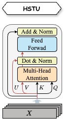
hstu的计算逻辑为： \(\text{FFN} \textcolor{red}(((\text{sigmoid}(Q \times K^T+bias) \odot mask) \times V) \odot (mask \times U)\textcolor{red}) + X\)

• Q、K、V的形状均为 [batch_size, num_heads, seq_len, head_dim]，经过mask后的U的形状为 [batch_size, seq_len, num_heads*head_dim]
• 对该结构有几种不同的理解
  • 视角1：本质上是resnet版的senet在序列特征上的适配。通过MTA产出各位置的权重，对（经过线性变换后的）原向量U做reweight；即让V去学特征重要度，但因为V只有当前位置的视角，建模能力有限，故通过QK的attention_weight实现更个性化的带权pooling。
  • 视角2（后续思考可以该视角为主）：高低阶特征交叉，DCN在序列特征上的适配。类似DCNv2的逻辑（用『左乘一个行向量（线性加权组合）的结果与要交叉的特征做哈达玛积 \(x_0 \odot (w^T x_0) + x_0\) 』来等价『与要交叉的特征做外积后的结果 内积一个列向量 \((x_0 x_0^T) w + x_0\) 』的操作），MHA完成线性加权组合的操作，与（经过线性变换后的）原向量U做哈达玛积，实现序列特征的隐式交叉。
• 使用时，若只基于该结构（类似于GR中的encoder-only结构），用用户的历史序列预测target(item)的action，user和item的交叉不够显式，只有隐式地将其它位置的信息线性加权到item上来，可能难以训好。

token-mixer

ID系统

离散ID

语义ID

向量量化变分自动编码器(VQ-VAE)

残差量化变分自动编码器RQ-VAE

局部敏感哈希(LSH)